What is a CNN

CNN are neural network that have layers called convolutional layers. They have some type of specialization for being able to pick out or detect patterns. This pattern detection is what makes CNNs so useful for image analysis.

Convolution

Convolution - operation that transforms an input into an output through a filter and a sliding window mechanism.

Convolution animation example: a convolutional filter, shaded on the bottom, is sliding across the input channel.

• Blue (bottom) - Input channel.
• Shaded (on top of blue) - 3x3 convolutional filter or kernel.
• Green (top) - Output channel.

For each position on the blue input channel, the 3 x 3 filter does a computation that maps the shaded part of the blue input channel to the corresponding shaded part of the green output channel.

Operation
At each step of the convolution, the sum of the element-wise dot product is computed and stored.

$$\begin{gathered} \begin{array}{r}{I}_{nput}=\left(\begin{array}{ccc}{a}_{11}& a_{12}& a_{13}\\ a_{21}& a_{22}& a_{23}\\ a_{31}& a_{32}& a_{33}\end{array}\right)\\ F_{ilter}=\left(\begin{array}{ccc}{b}_{11}& b_{12}& b_{13}\\ b_{21}& b_{22}& b_{23}\\ b_{31}& b_{32}& b_{33}\end{array}\right)\end{array} \\ Output=a_{11}{b}_{11}+a_{12}{b}_{12}+...+a_{33}{b}_{33} \end{gathered}$$

After this filter has convolved the entire input, we’ll be left with a new representation of our input, which is now stored in the output channel. This output channel is called a feature map.

Feature map - output channels created from the convolutions.

The word feature is used because the outputs represent particular features from the image, like edges for example, and these mappings emerge as the network learns during the training process and become more complex as we move deeper into the network.

Conv Layer

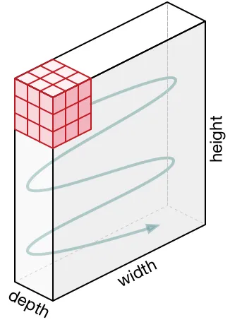
When adding a convolutional layer to a model, we also have to specify how many filters we want the layer to have.

The number of filters determines the number of output channels.

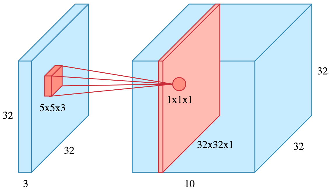
For example, if we apply 10 filters of size 5x5x3 to an input of size 32x32x3, we will obtain a 32x32x10 output, where each depth component (red slice in image) is a feature map.

Filters - allow the network to detect patterns, such as edges, shapes, textures, curves, objects, colors.

The deeper the network goes, the more sophisticated the filters become. In later layers, rather than edges and simple shapes, our filters may be able to detect specific objects like eyes, ears, hair or fur, feathers, scales, and beaks.

In even deeper layers, the filters are able to detect even more sophisticated objects like full dogs, cats, lizards, and birds.

Hyperparameters

1. Padding - add values “around” the image.
   • helps preserve the input’s spatial size (output size same as input), which allows an architecture designer to build deeper, higher performing networks.
   • can help retain information by conserving data at the borders of activation maps.
2. Kernel size - dimensions of the sliding window over the input.
   • massive impact on the image classification task.
   • small kernel size
     • able to extract a much larger amount of information containing highly local features from the input.
     • also leads to a smaller reduction in layer dimensions, which allows for a deeper architecture.
     • generally lead to better performance because able to stack more and more layers together to learn more and more complex features.
   • large kernel size
     • extracts _less information.
     • leads to a faster reduction in layer dimensions, often leading to worse performance.
     • better suited to extract larger features.
3. Stride - how many pixels the kernel should be shifted over at a time.
   • ↗️ stride ↘️ size of output
   • similar impact than kernel size
     • ↘️ stride ↗️ size of output + more features are learned because more data is extracted.
     • ↗️ stride ↘️ size of output + less feature extraction.

Most often, a kernel will have odd-numbered dimensions — like kernel_size=(3, 3) or (5, 5) — so that a single pixel sits at the center, but this is not a requirement.

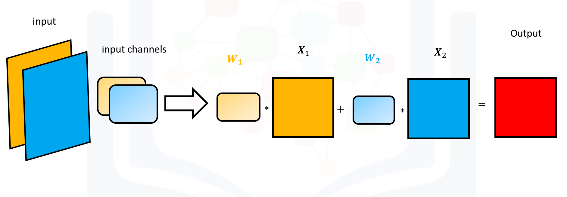
Conv2d with multiple input channels

For two inputs, you can create two kernels. Each kernel performs a convolution on its associated input channel. The resulting output is added together as shown:

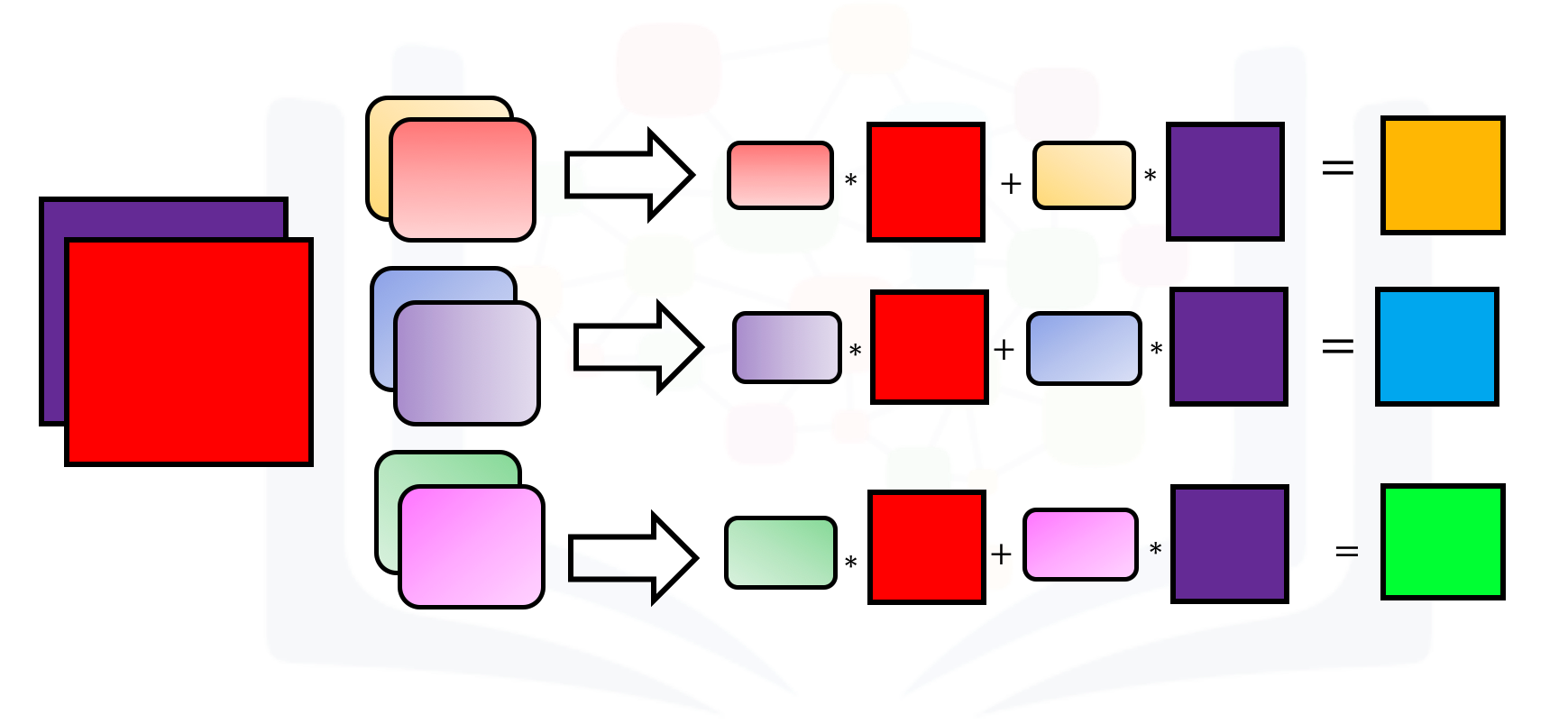
When using multiple inputs and outputs, a kernel is created for each input, and the process is repeated for each output. The process is summarized in the following image.

There are two input channels and 3 output channels. For each channel, the input in red and purple is convolved with an individual kernel that is colored differently. As a result, there are three outputs.

Parameters

$Parameters=(k_w\ast k_h\ast k_d+1)\ast C_{out}$

• $k_w$ = kernel width
• $k_h$ = kernel height
• $k_d$ = kernel depth (= input depth)
• $C_{out}$ = number of filters

Activation Function

In essence, a convolution operation produces a weighted sum of pixel values. Therefore, it is a linear operation. Following a convolution with another will just be a convolution.

Each element of the kernel is a weight that the network will learn during training.

However, part of the reason CNNs are able to achieve such tremendous accuracies is because of their non-linearity. Non-linearity is necessary to produce non-linear decision boundaries, so that the output cannot be written as a linear combination of the inputs. If a non-linear activation function was not present, deep CNN architectures would devolve into a single, equivalent convolutional layer, which would not perform nearly as well.

That is why we follow the convolution with a ReLU activation, which makes all negative values to zero.

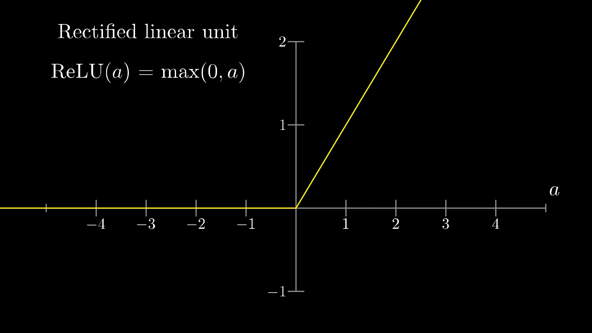
The ReLU activation function is specifically used as a non-linear activation function, as opposed to other non-linear functions such as Sigmoid because it has been empirically observed that CNNs using ReLU are faster to train than their counterparts.

Pooling Layer

Down-sampling operation that reduces the dimensionality of the feature map.

Purpose of gradually decreasing the spatial extent of the network, which reduces the parameters and overall computation of the network.

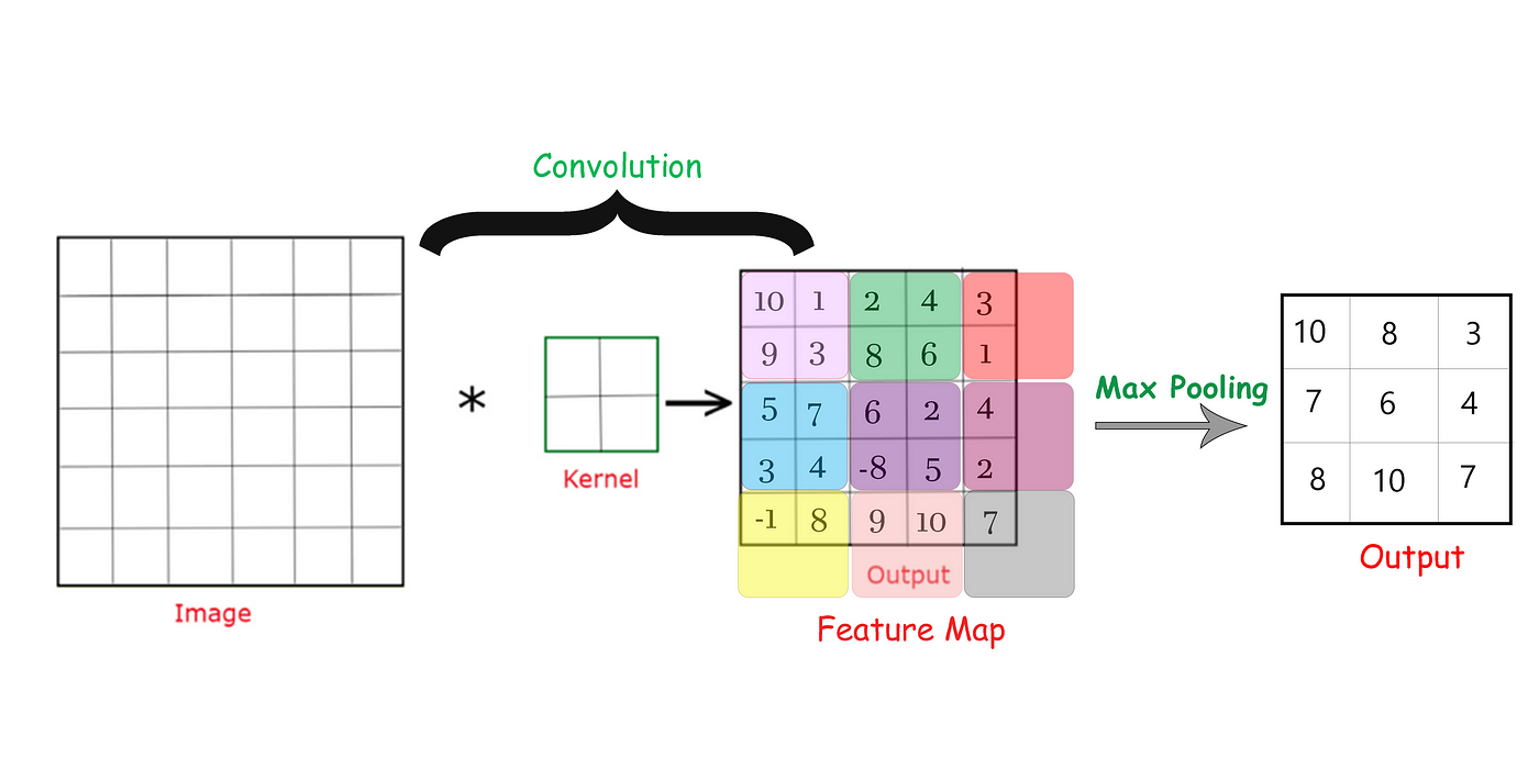
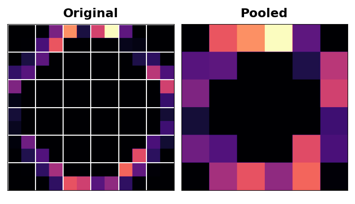
MaxPooling operation with a 2x2 kernel with (2,2) stride. We can think of each 2 x 2 blocks as pools of numbers.

Works like a convolution, but instead of computing the weighted sum, we return the Maximum value (MaxPooling) or the Average value (AvgPooling). As such, this layer doesn’t have any trainable parameters.

A little bit more in depth

After applying the ReLU function, the feature map ends up with a lot of ‘dead space’ that is, large areas containing only 0’s. Having to carry these 0 activations through the entire network would increase the size of the model without adding much useful information. Instead, we would like to condense the feature map to retain only the most useful part — the feature itself.

This in fact is what maximum pooling does. Max pooling takes a patch of activations in the original feature map and replaces them with the maximum activation in that patch.

When applied after the ReLU activation, it has the effect of ‘intensifying’ features. The pooling step increases the proportion of active pixels to zero pixels.

Translation Invariance

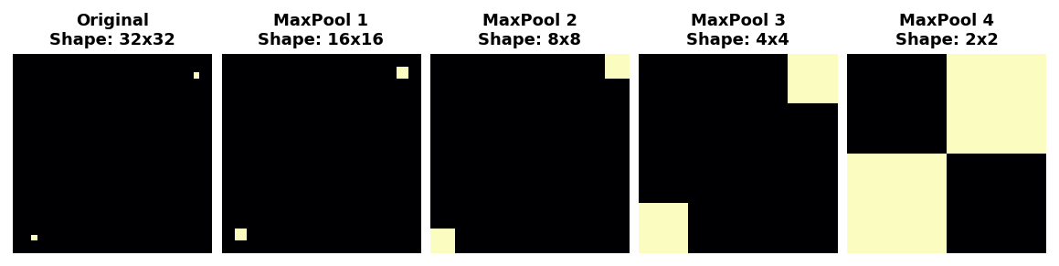
We called the zero-pixels ‘unimportant’. Does this mean they carry no information at all? In fact, the zero-pixels carry positional information. The blank space still positions the feature within the image. When MaxPool2D removes some of these pixels, it removes some of the positional information in the feature map. This gives a convnet a property called translation invariance. This means that a convnet with maximum pooling will tend not to distinguish features by their location in the image. (Translation is the mathematical word for changing the position of something without rotating it or changing its shape or size.)

Watch what happens when we repeatedly apply maximum pooling to the following feature map.

The two dots in the original image became indistinguishable after repeated pooling. In other words, pooling destroyed some of their positional information. Since the network can no longer distinguish between them in the feature maps, it can’t distinguish them in the original image either: it has become invariant to that difference in position.

In fact, pooling only creates translation invariance in a network over small distances, as with the two dots in the image. Features that begin far apart will remain distinct after pooling; only some of the positional information was lost, but not all of it.

This invariance to small differences in the positions of features is a nice property for an image classifier to have. Just because of differences in perspective or framing, the same kind of feature might be positioned in various parts of the original image, but we would still like for the classifier to recognize that they are the same. Because this invariance is built into the network, we can get away with using much less data for training: we no longer have to teach it to ignore that difference. This gives convolutional networks a big efficiency advantage over a network with only dense layers.

Parameters

Only reduces dimension, no parameters to be learned.

Flatten Layer

Converts a three-dimensional layer in the network into a one-dimensional vector to fit the input of a fully-connected layer for classification. Used after all Conv blocks so that we can fit our output to a fully connected layer.

Fully Connected Layer

Traditional feed-forward neural network that take the high-level features learned by convolutional layers and use them for final predictions.

Parameters

$Parameters=(inputunits\ast outputunits)+outputunits$

Regularization

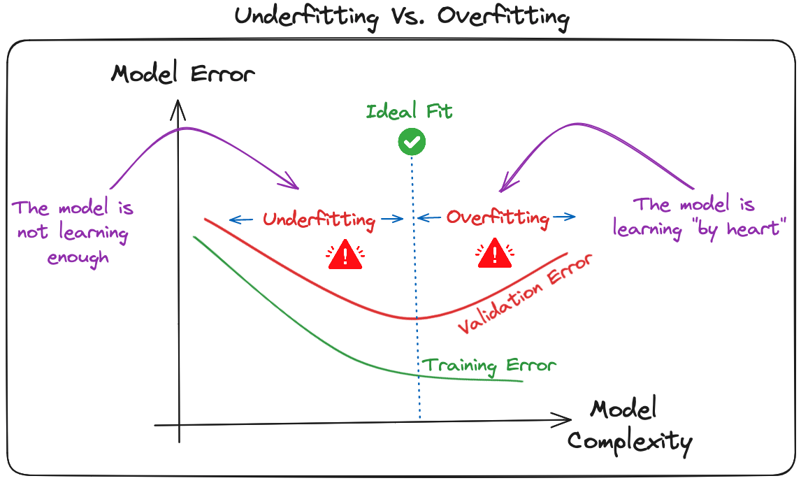
Deep learning models, especially CNNs, are particularly susceptible to overfitting due to their capacity for high complexity and their ability to learn detailed patterns in large-scale data.

Overfitting - model becomes too closely adapted to the training data, capturing even its random fluctuations. The model describes features that arise from noise or variance in the data, rather than the underlying distribution from which the data were drawn.

Several regularization techniques can be applied to mitigate overfitting in CNNs :

• Batch normalization: The overfitting is reduced at some extent by normalizing the input layer by adjusting and scaling the activations. This approach is also used to speed up and stabilize the training process.
• Dropout: This consists of randomly dropping some neurons during the training process, which forces the remaining neurons to learn new features from the input data.
• L1 and L2 normalizations: Both L1 and L2 are used to add a penalty to the loss function based on the size of weights. More specifically, L1 encourages the weights to be spare, leading to better feature selection. On the other hand, L2 (also called weight decay) encourages the weights to be small, preventing them from having too much influence on the predictions.
• Early stopping: This consists of consistently monitoring the model’s performance on validation data during the training process and stopping the training whenever the validation error does not improve anymore.
• Data augmentation: This is the process of artificially increasing the size and diversity of the training dataset by applying random transformations like rotation, scaling, flipping, or cropping to the input images.
• Noise injection: This process consists of adding noise to the inputs or the outputs of hidden layers during the training to make the model more robust and prevent it from a weak generalization.
• Pooling Layers: This can be used to reduce the spatial dimensions of the input image to provide the model with an abstracted form of representation, hence reducing the chance of overfitting.

More here.

---

📂 Ressources

📖 Articles
CNN Explainer
Introduction to CNNs by datacamp
Kaggle Computer Vision Course
Comprehensive Guide to CNNs
Convolution and ReLU
Batch Norm Explained Visually

📌Additional

Movement of a kernel.

❓ Questions
Why do we make convolutions on RGB images?
Why we use activation function after convolution layer in Convolution Neural Network?
Reason behind performing dot product on Convolutional Neural networks
What’s the purpose of using a max pooling layer with stride 1 on object detection