What is a neural network

Structure of a neural network

Neuron - a thing that holds a number (between 0.0 and 1.0), called the activation of that neuron.

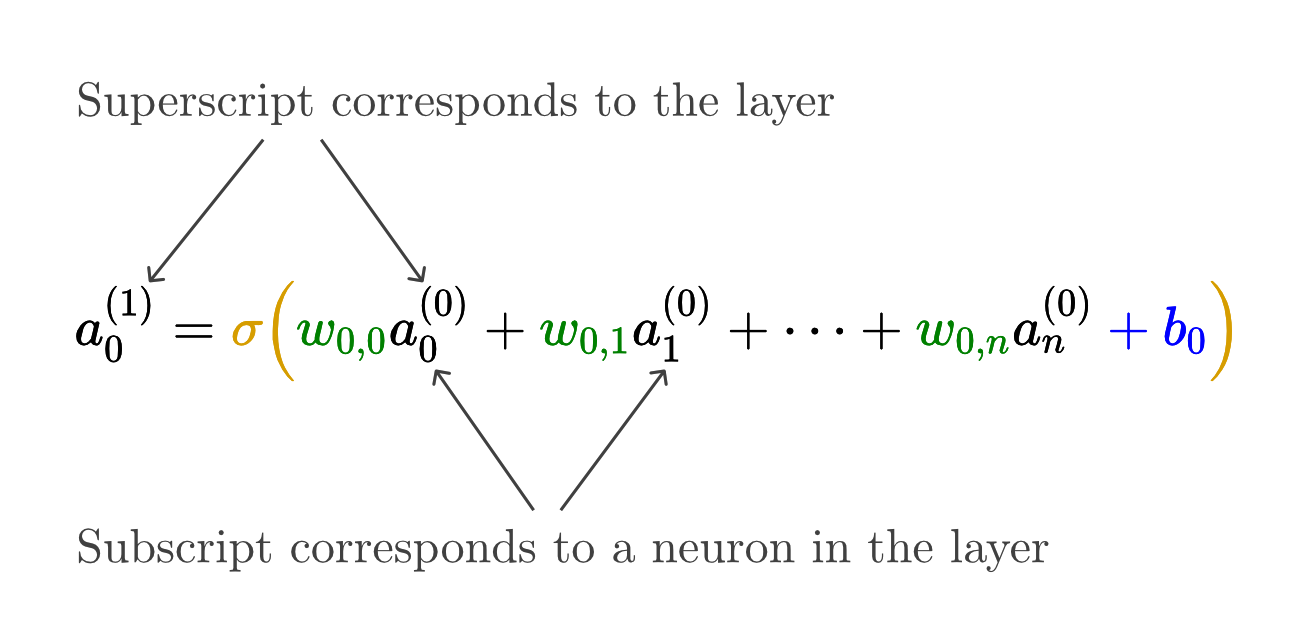
Each link between neurons indicates how the activation of each neuron in one layer, has some influence on the activation of each neuron in the next layer. However, not all these connections are equal. Determining how strong these connections are is really the heart of how a neural network operates.

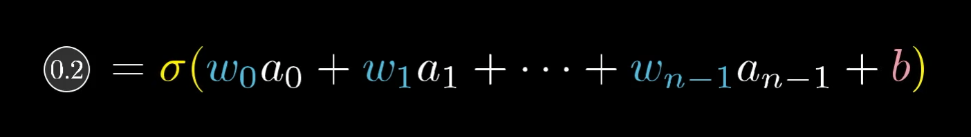
Activation Function - Function that squishes the weighted sum to be between 0.0 and 1.0.
Bias - how big the weighted sum needs to be before the neuron gets meaningfully active.

Gradient descent

learning = changing the weights and biases to minimize a cost function.

How the network learns

Cost function - cost difference between output predicted and expected.

The cost is small when the network confidently classifies this image correctly but large when it doesn’t know what it’s doing.

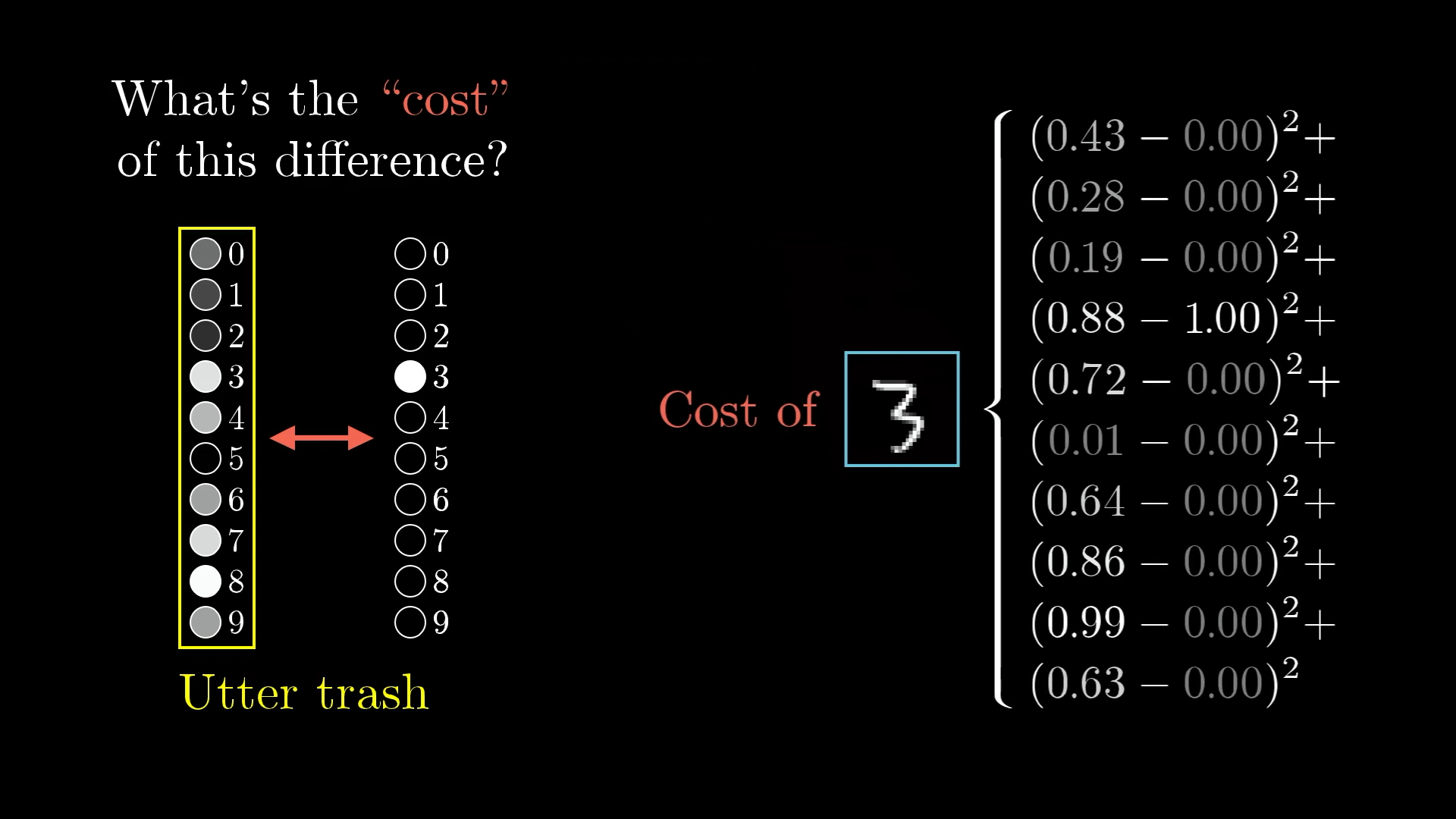
Exemple for one image : the “cost” is calculated by adding up the squares of the differences between what we got and what we want.

Cost of model - compute cost function over multiple examples and get the average cost.
• Input : weights and biases
• Output : one number
• Parameters : many training examples

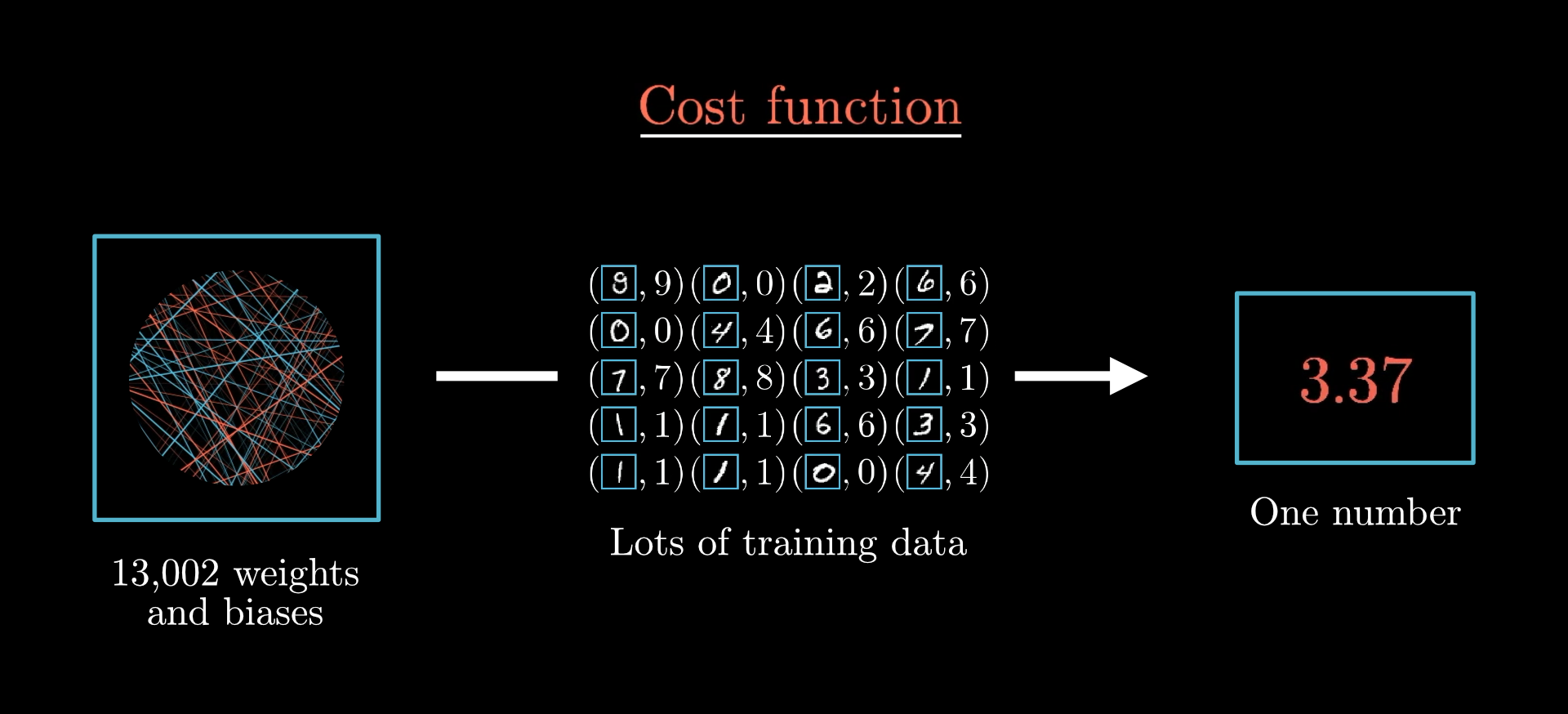
The cost function takes in the weights and biases of a network and uses the training images to compute a “cost,” measuring how bad the network is at classifying those training images.

Minimizing the cost
The goal is to minimize the cost so our network performs better. From our actual random position, which direction should you step in this input space to decrease the output of the function most quickly.

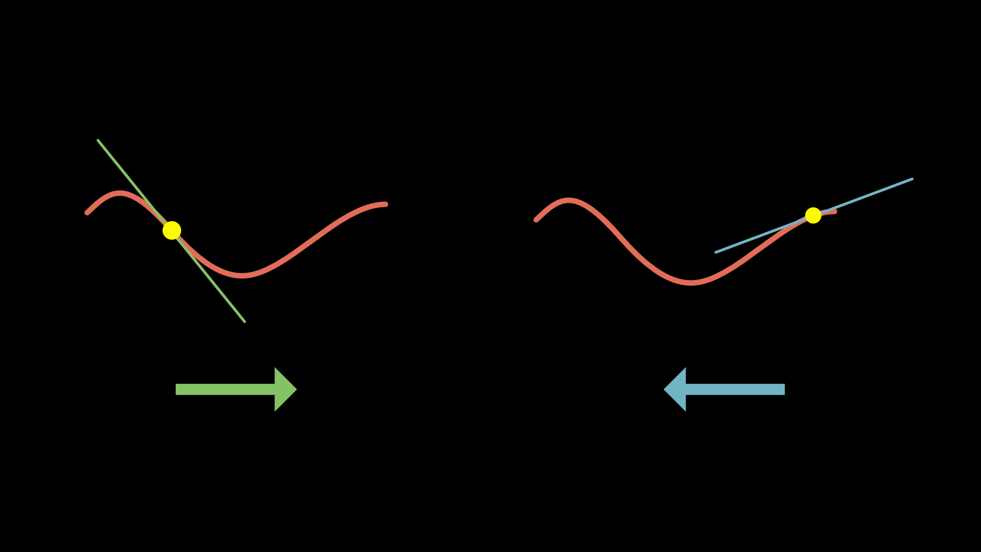
*By following the slope (moving in the downhill direction), we approach a local minimum. Also, as the slope gets shallower, take smaller steps to avoid overshooting the minimum.

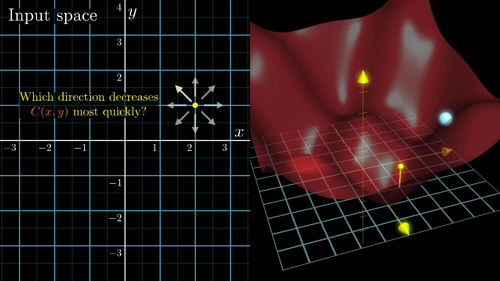
We can imagine minimizing a function that takes two inputs (which is still not 13,002 inputs, but it’s one step closer). Starting with a random value, look for the downhill direction and repeatedly move that way.

Gradient - direction (vector) of steepest increase.

Since we are interested in steepest decrease, we’ll be interested in the negative gradient.

Gradient descent - algorithm to minimize the cost function aka process of using gradients to find the minimum value of the cost function.

1. Compute gradient.
2. Small step in the negative gradient direction.
3. Repeat.

$Inpractice,eachstepwilllooklike-\eta \nabla Cwhere\eta isknownasthe\text{learningrate}.$

The larger the learning rate, the bigger the steps and vice-versa.

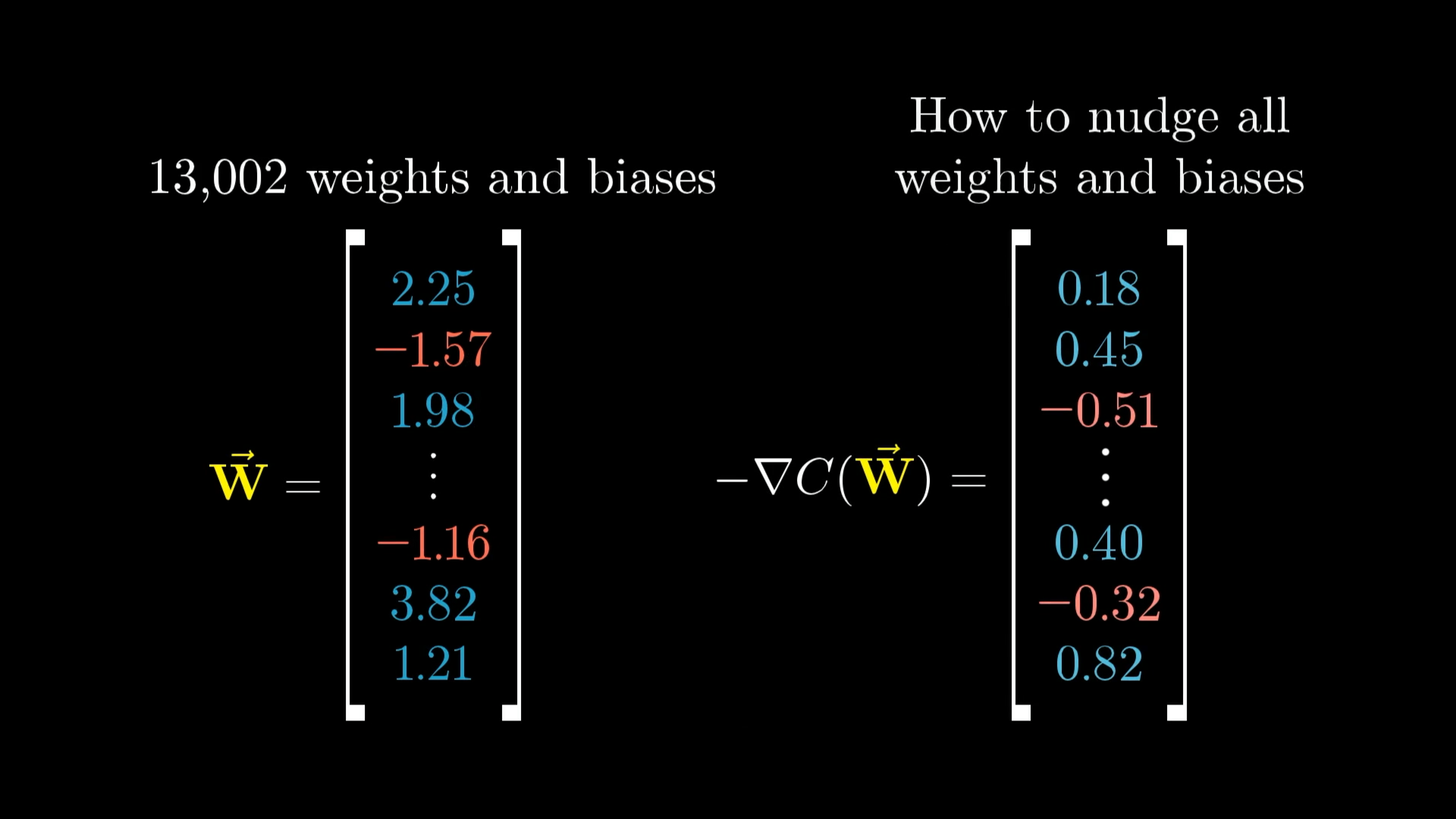
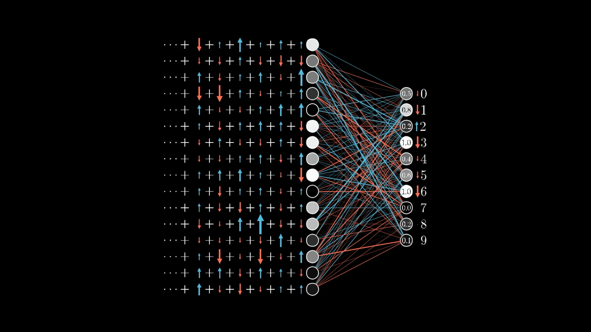
The vector on the left is a list of all the weights and biases for the entire network. The vector on the right is the negative gradient, which is just a list of all the little nudges you should make to the weights and biases (on the left) in order to move downhill.

Stochastic gradient descent - refers to the use of a random subset of the data when computing the gradient. We instead get an estimate of the actual gradient (computed from the entire data set).

Stochastic vs Batch

Standard gradient descent and batch gradient descent were originally used to describe taking the gradient over all data points, and by some definitions, mini-batch corresponds to taking a small number of data points (the mini-batch size) to approximate the gradient in each iteration. Then officially, stochastic gradient descent is the case where the mini-batch size is 1.

However, perhaps in an attempt to not use the clunky term “mini-batch”, stochastic gradient descent almost always actually refers to mini-batch gradient descent, and we talk about the “batch-size” to refer to the mini-batch size. Gradient descent with > 1 batch size is still stochastic, so I think it’s not an unreasonable renaming, and pretty much no one uses true SGD with a batch size of 1, so nothing of value was lost.

Ref

With these mini-batches, which only approximate the gradient, the process of gradient descent looks more like a drunk man stumbling aimlessly down a hill but taking quick steps rather than a carefully calculating man who takes slow, deliberate steps downhill.

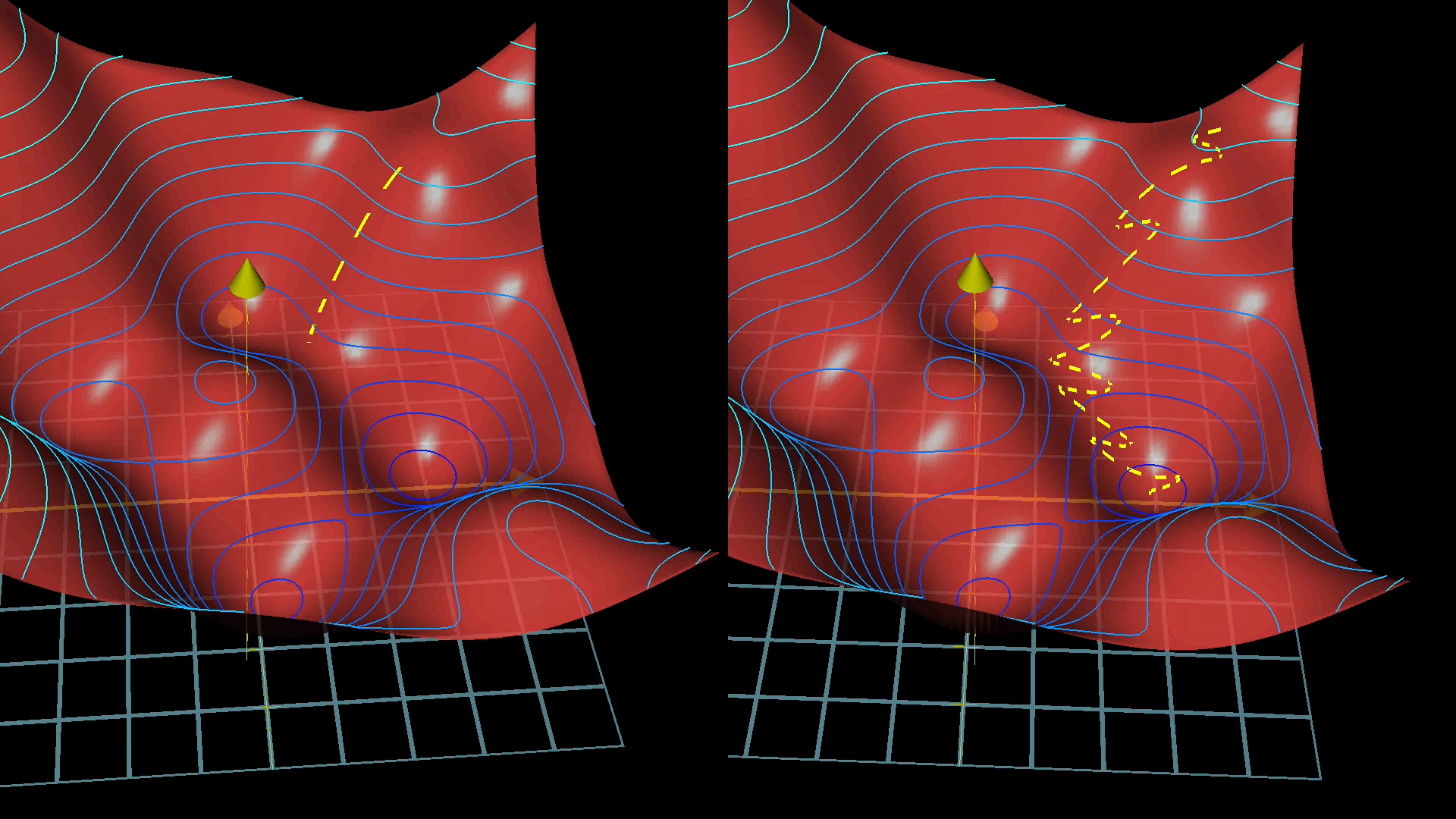
Using mini-batches means our steps downhill aren’t quite as accurate, but they’re much faster.

Backward Propagation

Backward propagation - algorithm that computes the negative gradient.

🔎 One example, one neuron

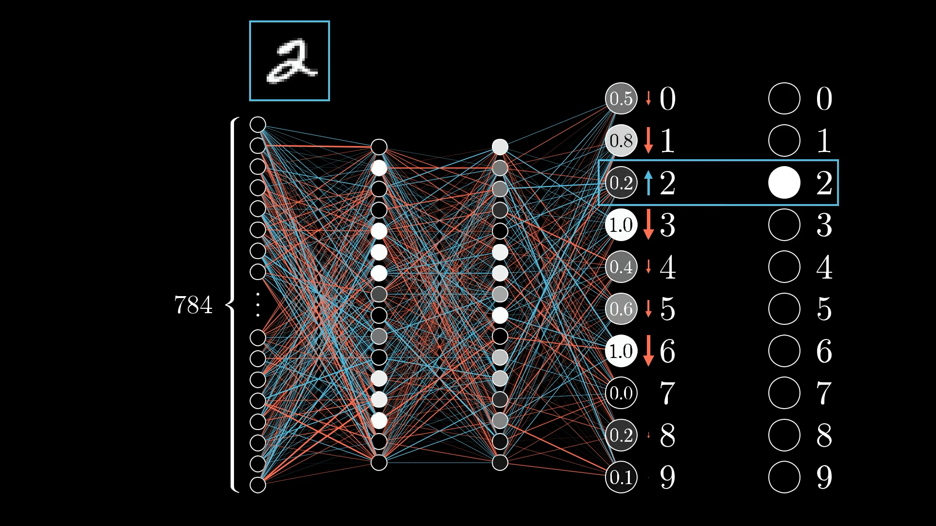
We want the digit 2 neuron’s value to be nudged up while all the others get nudged down.

Activation value of the neuron :

3 ways to increase this activation:

1. Increase the bias

Simplest way to change its activation. Unlike changing the weights or the activations from the previous layer, the effect of a change to the bias on the weighted sum is constant and predictable.

2. Increase the weights

The connections with the brightest neurons from the preceding layer have the biggest effect since those weights are multiplied by larger activation values. So increasing one of those weights has a bigger influence on the cost function than increasing the weight of a connection with a dimmer neuron.

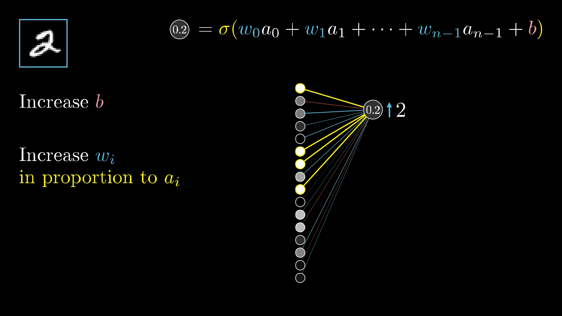
To get the most bang for your buck, adjust the weights in proportion to their associated activations.

3. Changing the activations

Namely, if everything connected to that digit-2 neuron with a positive weight was brighter, and if everything connected with a negative weight was dimmer, that digit-2 neuron would be more active.

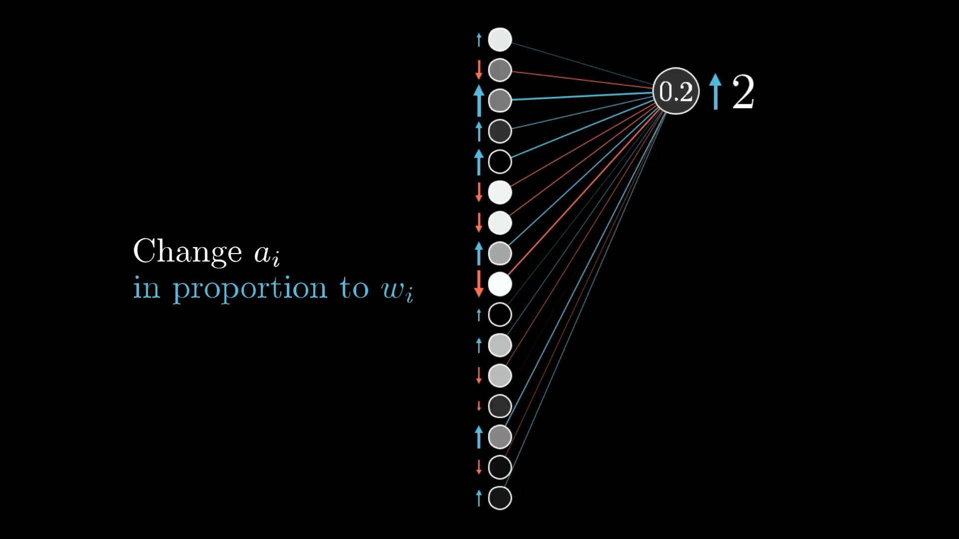
Just like changing weights in proportion to activations, you get the most bang for your buck by increasing activations in proportion to their associated weights.

↪️ However, we can’t directly influence the activations in the previous layer, but we can change the weights and biases that determine their values.

🧩 One example, all neurons

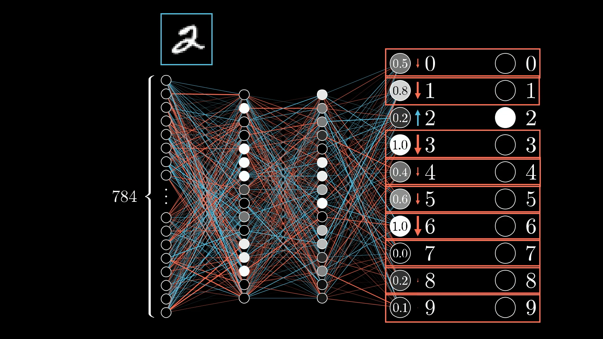
We want to adjust all these other output neurons too, which means we will have many competing requests for changes to activations in the previous layer.

It’s impossible to perfectly satisfy all these competing desires for activations in the second layer. The best we can do is add up all the desired nudges to find the overall desired change.

🌎 All examples

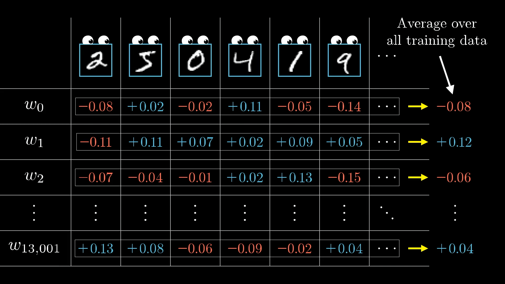
Each training example has its own desire for how the weights and biases should be adjusted, and with what relative strengths. By averaging together the desires of all training examples, we get the final result for how a given weight or bias should be changed in a single gradient descent step.

The result of all this backpropagation is that we’ve found (something proportional to) the negative gradient.

Calculus

📂 Ressources

📖 But what is a neural network? by 3blue1brown.
📖 Gradient descent, how neural networks learn by 3blue1brown.
📖 What is backpropagation really doing? by 3blue1brown.
📖 Backpropagation calculus by 3blue1brown.