RAG from Scratch

Overview

RAG (Retrieval-Augmented Generation) allows an LLM to use external data (often private) to answer questions.

LLMs are trained on large amounts of public data, but most useful data in real-world applications is not included in training (e.g., company docs, personal data, internal databases).
RAG solves this by injecting relevant information at inference time.

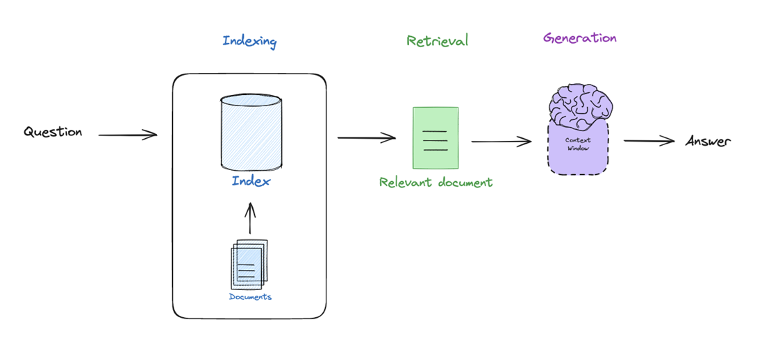
Core pipeline:

1. Indexing → Prepare and structure documents
2. Retrieval → Find relevant information
3. Generation → Produce an answer using retrieved data

Key intuition:
RAG = LLM + Search system

Indexing

Convert raw documents into a format that can be efficiently searched.

Process:

• Load documents
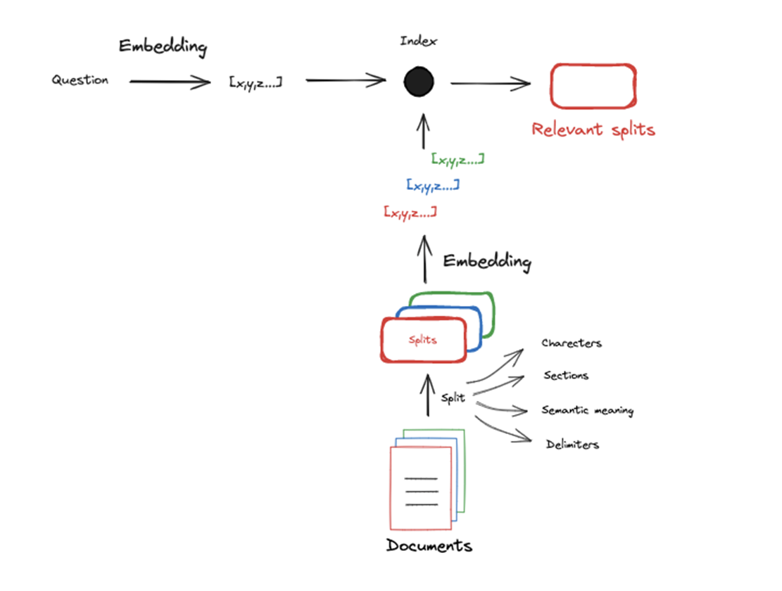
• Split them into smaller chunks
• Convert each chunk into a vector representation (embedding)
• Store them in a vector database

Text cannot be easily compared directly. Hence many approaches have been developed to compress text documents into numerical representation, allowing similarity computations.
Two main approaches:

• Sparse vectors (e.g., TF-IDF): based on word frequency
• Dense vectors (embeddings): capture semantic meaning

Modern RAG systems mainly use dense embeddings.

Chunking (important):

Because LLMs and embedding models have a limited context window, often documents are split up before they are embedded.

• Embedding models have input size limits.
• Smaller chunks improve retrieval precision.

Retrieval

Given a query, retrieve the most relevant document chunks.

Process:

• Convert the query into an embedding
• Compare it with stored document embeddings
• Retrieve the closest ones

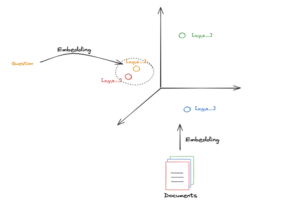
Documents with similar meanings are close in vector space. Since the question also is embedded, retrieval is essentially a nearest-neighbor search in embedding space.

K parameter

Defines how many documents to retrieve

• Small K → precise but limited context
• Large K → more context but more noise

📁 Ressources
📖 Vector Search - Hierarchical Navigable Small World (HNSW)
📌 https://superlinked.com/vector-db-comparison
📝 LangChain - Vectorstores

Generation

Use retrieved documents to generate a grounded answer.

Process:

• Take retrieved chunks
• Insert them into the LLM prompt
• Generate the answer

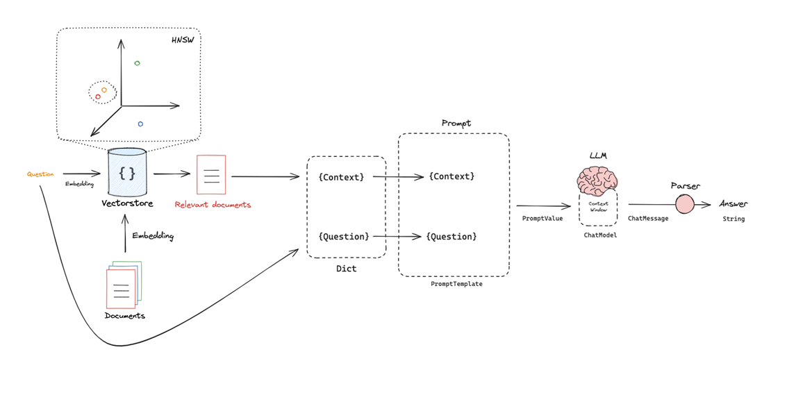
This uses the the idea of a prompt, which is a template that includes placeholders that we can popular with our particular retrieved docs and question. Typically includes:

• Context (retrieved documents)
• Question (user input)

Important detail

The LLM does not access the database directly : it only sees what is placed in its context window. Implications :

• Missing relevant documents → incorrect answer
• Irrelevant documents → hallucinations or confusion
• Too many documents → context overflow

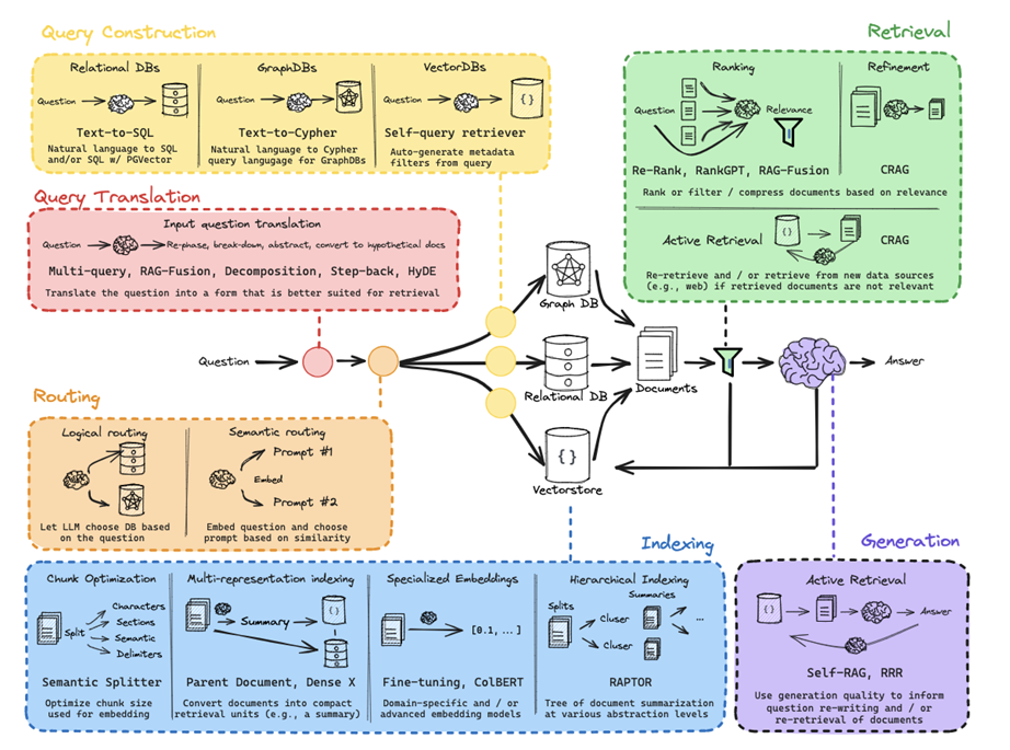
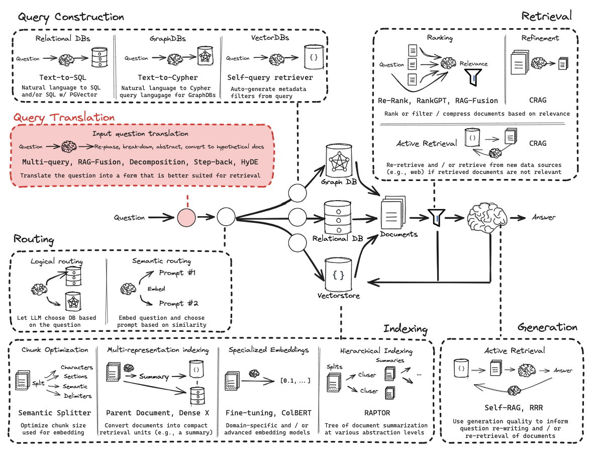
Query Translation

The goal is to transform a user’s raw question into a format that improves the chances of finding the right documents.

User queries are often:

• Ambiguous
• Poorly phrased
• Misaligned with document wording

Since retrieval depends on semantic similarity, a bad query leads to poor results.

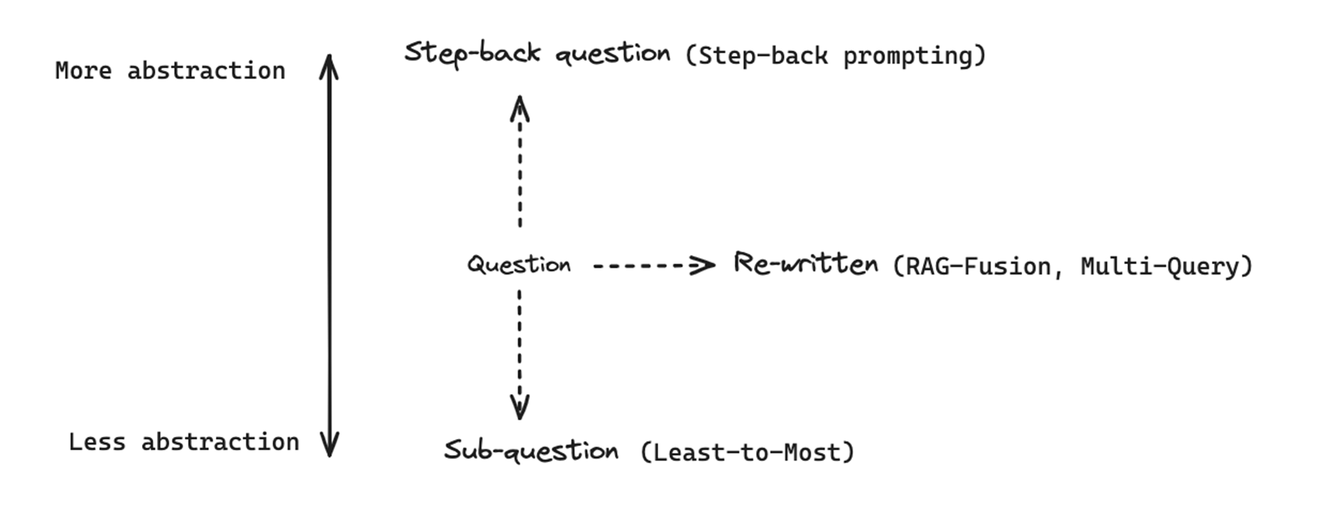
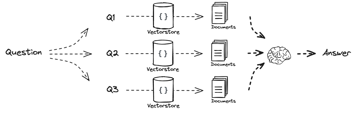
Re-written : Multi-query approach

Improve retrieval by rewriting the user query.

• Generate multiple variations of the original query
• Perform retrieval for each variation
• Combine all retrieved documents

Instead of relying on a single query, we explore multiple semantic directions. Different question phrasings lead to different embeddings, which in turn lead to a better chance of matching the relevant documents for our initial query.

Pipeline:

1. Original query
2. Generate multiple reformulations
3. Retrieve documents for each
4. Merge results
5. Generate final answer

Re-written : RAG Fusion

Improves retrieval robustness by combining multiple query reformulations with a smarter ranking strategy.

• Generate multiple query reformulations
• Perform retrieval for each query
• Additional step: Aggregate and re-rank results using RRF
• Pass final ranked documents to the LLM

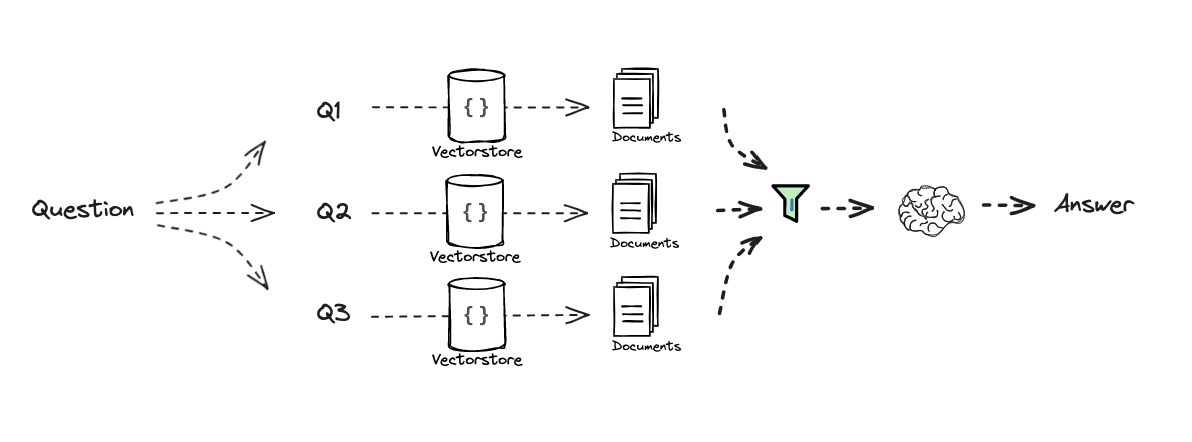
The key difference lies in how results are combined (i.e. Retrieval step). Rather than simply merging all retrieved documents, RAG Fusion applies Reciprocal Rank Fusion (RRF), a ranking method that prioritizes documents that consistently appear at the top across multiple retrievals. This helps filter noise and emphasize the most reliable results.

This approach is especially useful when retrieval results are diverse or when querying across multiple sources, as it produces a more stable and relevant final context.

Sub-question : Decomposition (Least-to-Most, IR-CoT)

Handle complex questions by breaking them into simpler sub-questions.

Instead of retrieving information for a single query, decomposition splits the original question into multiple sub-problems. Each sub-question can then be answered individually, making the overall problem easier to solve.

Two main strategies emerge:

• Sequential decomposition:
  Sub-questions are answered one after another, with each answer being used as additional context for the next. This creates a reasoning chain where knowledge is progressively accumulated.
• Parallel decomposition:
  Sub-questions are independent and can be answered separately. Their answers are then combined at the end.
  

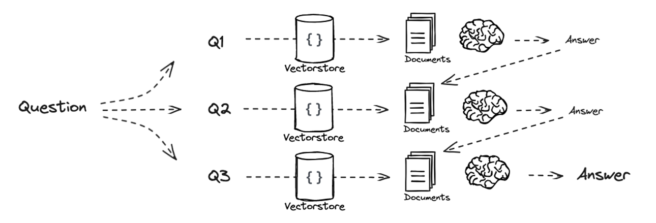
This graph shows sequential decomposition. For parallel decomposition, there would be no answer being linked into another question’s prompt, they would all directly be input of an LLM.

This method is closely related to chain-of-thought reasoning, but with retrieval integrated at each step, ensuring that intermediate answers are grounded in external data.

It is particularly effective for multi-hop questions, where the final answer depends on several pieces of information that must be connected.

Step-back question : Step-Back Prompting

Step-back prompting follows the opposite direction of decomposition by making the query more abstract instead of more detailed. The idea is to reformulate the original question into a broader, higher-level question that captures the underlying concept behind it.

This is typically done using few-shot prompting, where the model is shown examples of specific questions paired with their more general counterparts. Given a new query, the model generates a “step-back” version that is less tied to surface details and more focused on general knowledge.

Retrieval is then performed both on the original question and on the abstracted version. The retrieved documents from both perspectives are combined and provided to the model for answer generation. This allows the system to leverage both precise and conceptual information.

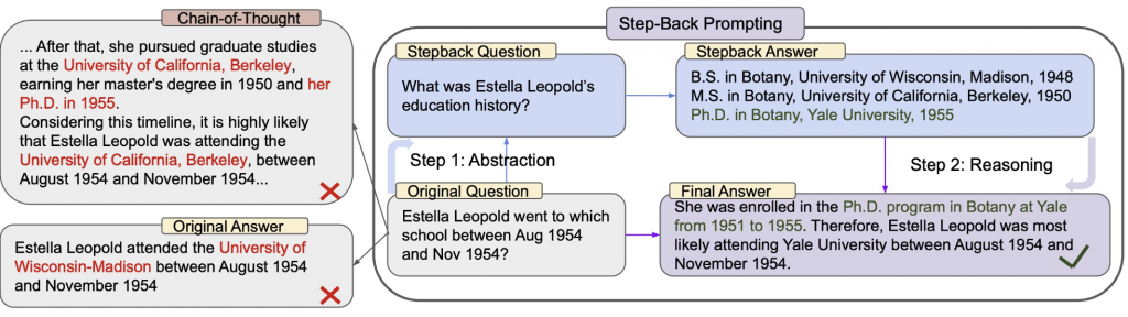
This approach is particularly useful in domains where understanding broader concepts is necessary to answer specific questions, such as technical documentation or educational content.

HyDE (Hypothetical Document Embeddings)

HyDE (Hypothetical Document Embeddings) addresses a fundamental mismatch in RAG systems: queries and documents are structurally different. Queries are typically short and sometimes vague, while documents are longer and more detailed. This difference can make similarity search less effective.

To overcome this, HyDE generates a hypothetical document that answers the user’s question, using the LLM’s internal knowledge. This generated passage is then embedded and used as the query for retrieval, instead of the original question.

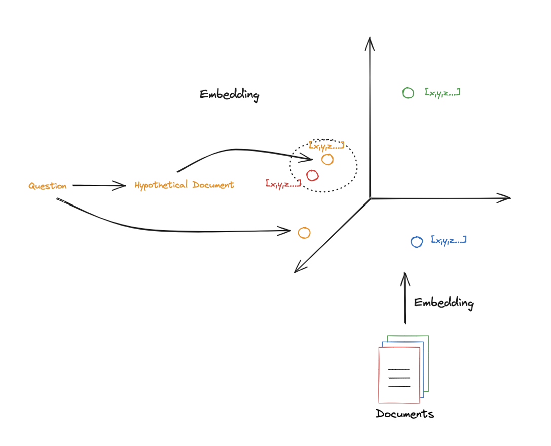
The intuition is that this synthetic document is closer in structure and semantics to real documents in the database, which improves the quality of similarity search. In embedding space, it is often positioned nearer to relevant documents than the raw query itself.

Once relevant documents are retrieved using this hypothetical document, they are passed, along with the original question, to the generation step.

Info

An important advantage of this approach is its flexibility : the prompt used to generate the hypothetical document can be adapted to the domain (e.g., scientific writing, technical explanations), which can further improve retrieval performance.

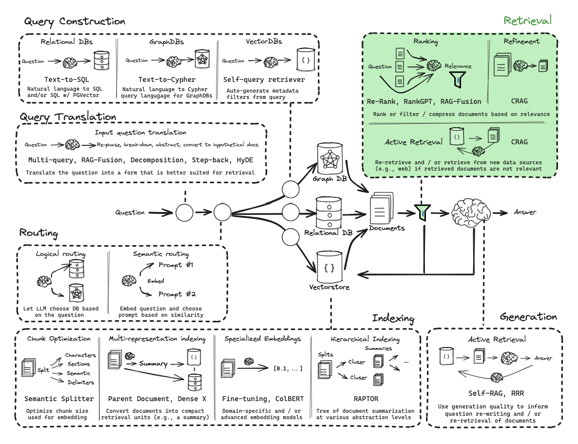
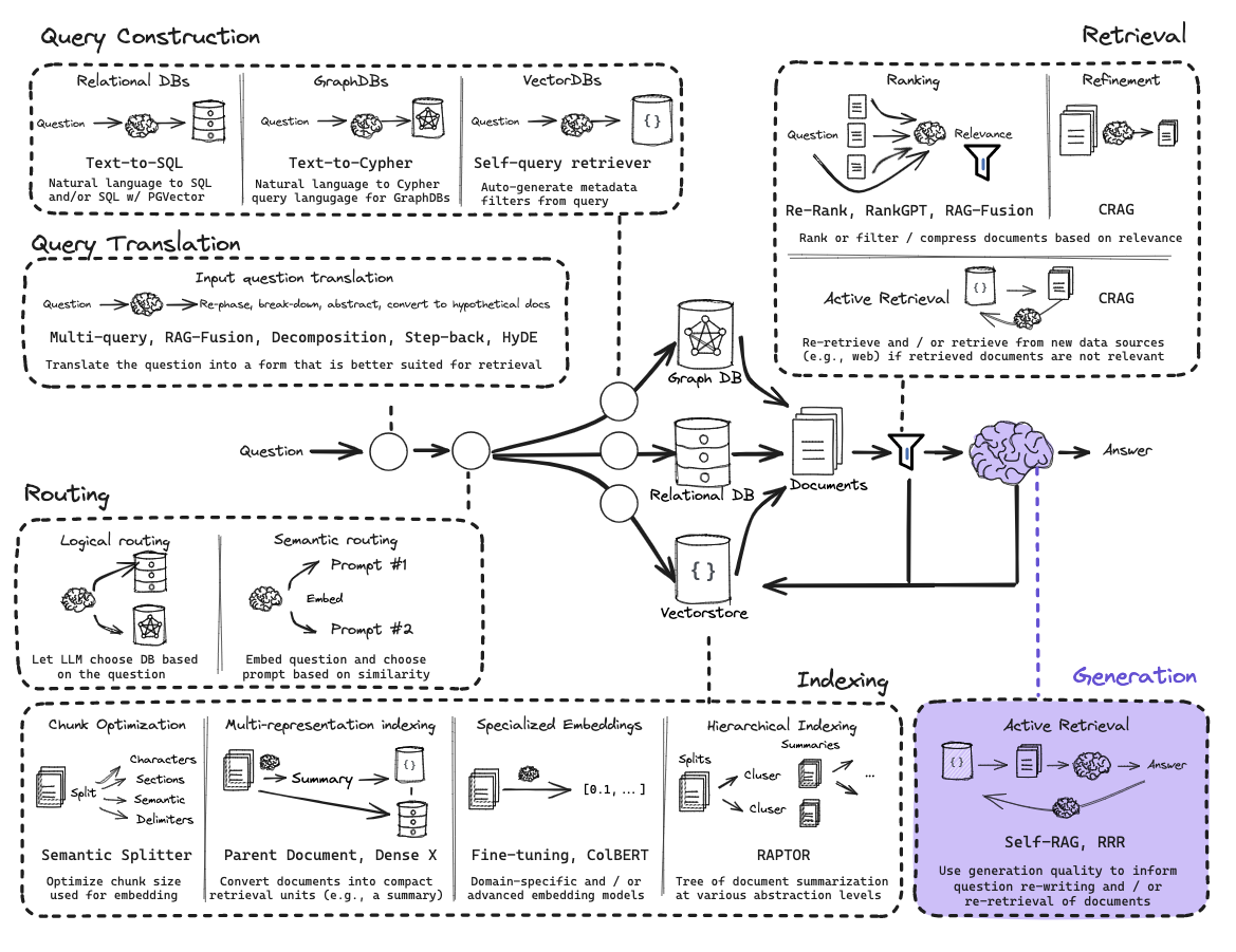
Routing

Routing is the process of directing a user’s query to the most appropriate data source or processing path. It usually follows Query Translation (where the question is refined or decomposed).

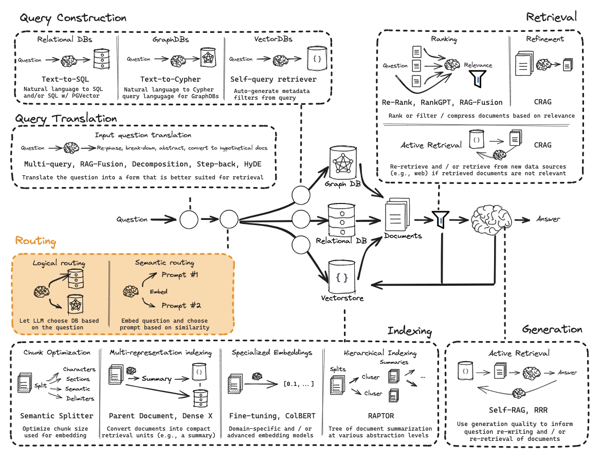
Two primary types of routing:

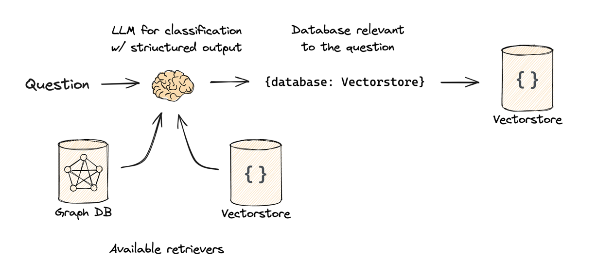
1. Logical Routing
   • Mechanism: The LLM is given descriptions of various data sources (e.g., a Vector Store, a Relational SQL DB, and a Graph DB).
   • Logic: The LLM “reasons” about the content of the user’s question and classifies it to determine which database is best suited to answer it.
   • Use Case: Choosing between different programming language documentations (e.g., routing a Python question to the Python docs and a JS question to the JS docs).

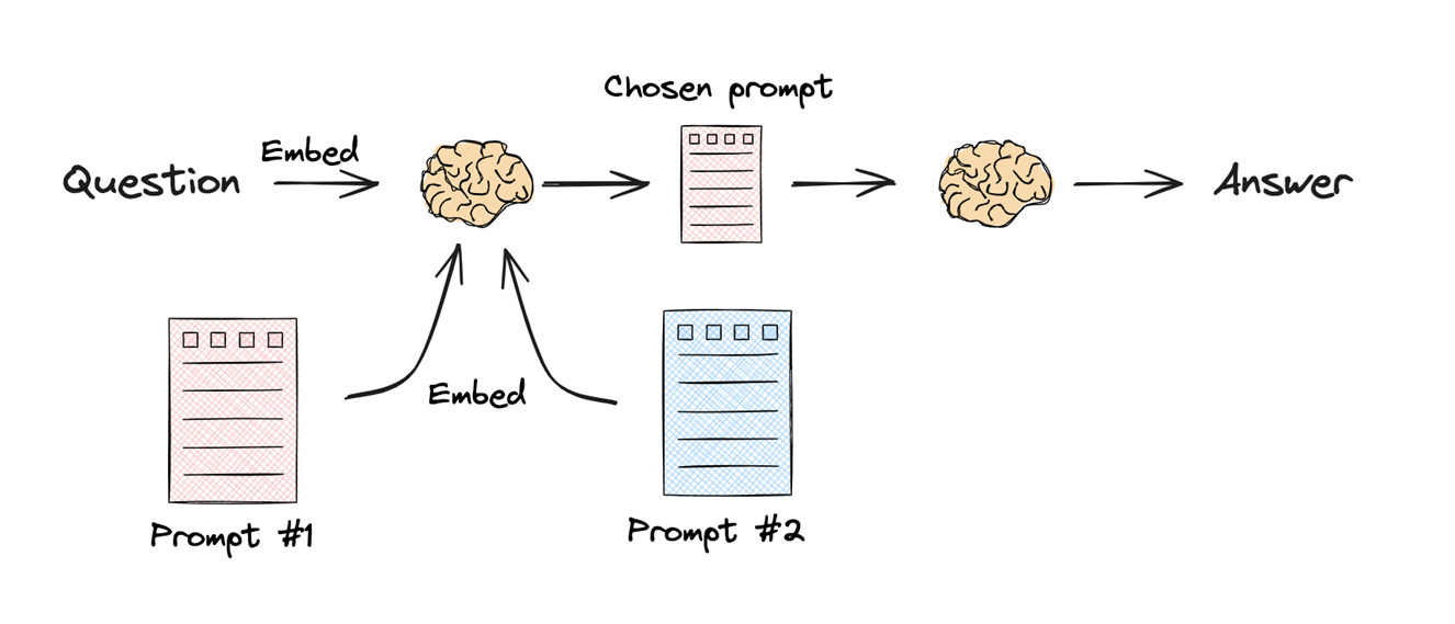
2. Semantic Routing
   • Mechanism: Both the query and the potential “destinations” (like specific prompts or topic categories) are turned into embeddings.
   • Logic: The system calculates the similarity between the query embedding and the destination embeddings. The query is routed to the destination with the highest similarity score.
   • Use Case: Matching a question about “Black Holes” to a “Physics Prompt” rather than a “Math Prompt” based purely on vector similarity.

Why Route?

Routing prevents “wasting” the query on irrelevant databases, ensuring that the retrieval step is focused on the most specialized and high-quality data source available for that specific topic.

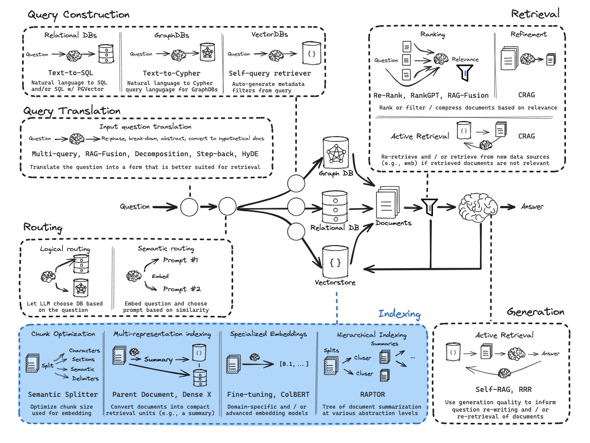
Query Construction

Query Construction is the process of converting an unstructured natural language question into a structured query (Domain Specific Language) that a database can understand.

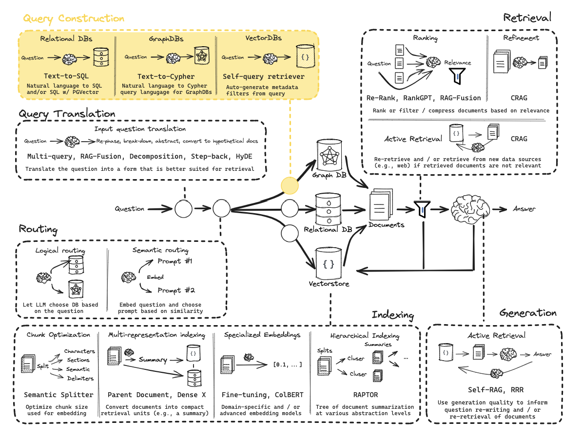
While vector stores are great at semantic (similarity) search, they often struggle with specific constraints like dates or exact counts. Query Construction solves this by generating Metadata Filters.

Problem: If a user asks for “videos published after 2024,” a standard vector search looks for the meaning of that sentence but might ignore the strict date constraint.

• Schema Definition: You define a structured model (e.g., using Pydantic) that represents the available metadata in your database (e.g., publish_date, view_count, video_length).
• Structured Output: The LLM takes the natural language query and “maps” it into this schema.
• Result: The user’s question is transformed into a search that combines:
  1. Semantic Search: Finding chunks related to the topic.
  2. Structured Filter: A hard constraint (e.g., date > 2024) applied to the results.

Example

1. User Input: “Find me tutorials on RAG published before 2024.”
2. LLM Processing: The LLM identifies “RAG” as the search term and “before 2024” as a metadata filter.
3. Output: A structured object containing search_term: “RAG” and filter: { “date”: { “$lt”: 2024 } }.
4. Database Execution: The Vector DB returns only the relevant “RAG” chunks that also meet the date requirement.

Indexing

Indexing is the process of transforming and storing documents in a structured, searchable format (e.g., embeddings in a vector database) so they can be efficiently retrieved later.

Multi-Representation

This technique challenges the traditional RAG assumption that the unit you search for must be the same as the unit you feed to the LLM.

In standard RAG, you split a document into chunks, embed those chunks, and send the retrieved chunks to the LLM. Multi-Representation Indexing decouples these steps.

The Retrieval Unit (i.e. “Summary”) - You use an LLM to create a condensed “proposition” or summary of each document split. This summary is optimized for retrieval : it contains the dense keywords, core themes, and “big ideas” that a user is likely to search for. You embed and store these in the Vector Store.

The Storage Unit (i.e. “Full Doc”) - You store the original, full-length, un-summarized documents in a separate Document Store (linked by a unique ID to the summaries).

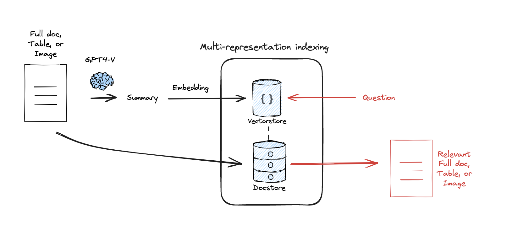
1. Search: The user query is compared against the summaries in the Vector Store.
2. Pointer: When a summary is “hit,” the system uses its ID to look up the full document in the Doc Store.
3. Generation: The LLM receives the entire, high-context document to generate an answer.

Why use this?

• Long-Context LLMs: Modern LLMs can handle 100k+ tokens. Sending them a tiny, fragmented chunk is often counterproductive.
• Retrieval Accuracy: It is mathematically easier to match a query to a dense summary than to a noisy, 500-word chunk of raw text.

RAPTOR: Recursive Abstractive Processing for Tree-Organized Retrieval

This technique builds a hierarchical representation of the data (like a tree of summaries).

RAPTOR addresses the level of abstraction problem in RAG. Standard retrieval is great for specific facts but terrible at thematic or holistic questions.

Example : if you have 100 documents about LangChain and a user asks, “What is the overall philosophy of this library?”, a standard retriever might grab 3 specific code-heavy chunks. These chunks are “low-level” and cannot answer a “high-level” question.

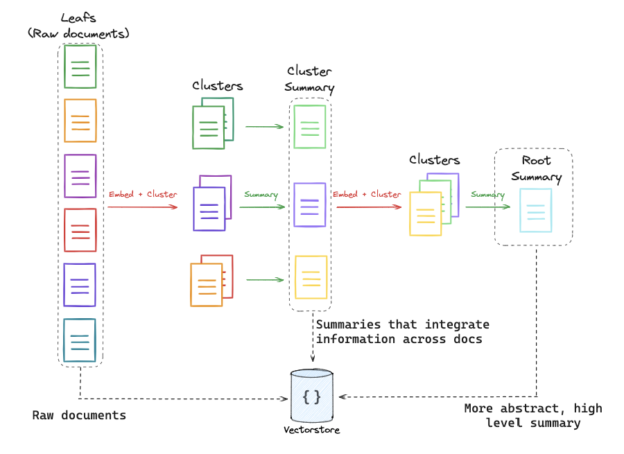
RAPTOR builds a pyramid of information :

1. Leaf Nodes: These are your raw document chunks at the bottom.
2. Clustering: The system clusters similar chunks together using embedding similarity.
3. Summarization: An LLM summarizes each cluster. These summaries become a “middle layer” of the tree.
4. Recursion: The process repeats. The middle-layer summaries are themselves clustered and summarized into a “top layer” (a global summary).

Crucially, RAPTOR doesn’t just search the top. It indexes every level of the tree (raw chunks + mid-summaries + top-summaries) into a single Vector Store.

Why use this?

• Multi-Granular Questions : If a user asks a specific question, the system retrieves a leaf (raw chunk). If they ask a global question, the system retrieves a summary node.
• Contextual Breadth : It allows the system to retrieve information that was originally spread across dozens of documents but has been synthesized into a single summary.

ColBERT: Contextualized Late Interaction

ColBERT is a move away from “Bi-Encoders” (standard embeddings) toward a more nuanced token-level similarity model.

Standard embedding models are compressors. They take a 512-token chunk and squeeze all that meaning into one single vector. This often loses the fine-grained nuance or specific needle in a haystack keywords.

Instead of one vector per document, ColBERT creates a vector for every single token in the document (and the query).

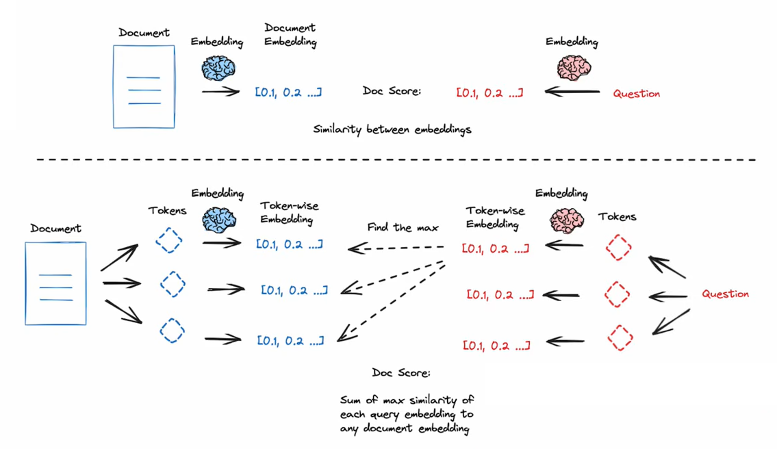
1. Multi-Vector Representation: A document isn’t a point in space; it’s a collection of points (one for each word/token).
2. MaxSim (Maximum Similarity): When a user asks a question, the system looks at each token in the query and finds the strongest match among all tokens in the document.
3. Summation: It adds up these “maximum similarities” to calculate a final score for the document.

By waiting until the very last second to compare individual query tokens to individual document tokens (Late Interaction), the model captures how words interact in context much better than a single-vector compression ever could.

Why use this?

• High Precision: It is significantly more accurate at finding specific information than standard cosine similarity search.
• Nuance: It understands that the word “Bank” in a query about “river banks” should only match tokens in documents that also use “bank” in a geographical context.

GraphRAG vs. VectorRAG (Global Intelligence)

While Lance Martin focused on VectorRAG (Semantic Similarity), the biggest 2026 advancement is GraphRAG, which solves the “Aggregation” problem.

VectorRAG is local. It is excellent at answering: “What is the height of the Eiffel Tower?”
It fails at answering global questions: “What are the recurring themes across all 5,000 of our customer support tickets from 2025?”
VectorRAG would just find 5 tickets that look like the question, missing the other 4,995.

GraphRAG doesn’t just store text; it extracts Entities (People, Companies, Tech) and Relationships (X works for Y; A is a feature of B).

• Mechanism 1: Community Summarization. The system clusters the Knowledge Graph into “Communities” (e.g., a “Security Community,” a “Billing Community”). An LLM pre-writes a summary for every community.
• Mechanism 2: Global Traversal. When you ask a broad question, the system looks at the Summaries of the Communities rather than individual text chunks.

When to use which?

Use Case	VectorRAG (Local)	GraphRAG (Global)
Question Type	Specific facts/details.	Thematic/Aggregated trends.
Data Type	Plain text, unorganized.	Highly connected data (Legal, Medical).
Retrieval Unit	Top $K$ most similar chunks.	Relevant “Nodes” and “Communities.”
Theoretical Strength	Semantic Similarity.	Structural Intelligence.

Hybrid Search (The 2026 Standard)

Today’s most advanced systems use Hybrid Search. They perform a Vector Search for the “details” and a Graph Search for the “context,” combining both results before generating the final answer.

Retrieval

Retrieval is the step where the system searches that index to find the most relevant documents or chunks to provide context for answering a given query.

CRAG : Corrective Retrieval-Augmented Generation

CRAG is a strategy designed to handle the reliability problem in RAG. In a basic RAG pipeline, the system blindly trusts whatever the retriever returns. CRAG introduces a self-correction mechanism to evaluate and supplement retrieval.

Traditional linear RAG follows a simple pipeline where documents are retrieved and then used to generate an answer, but it can fail when the retrieved information is irrelevant, leading to hallucinations or poor outputs. A more robust approach is Active RAG, which introduces a state machine based workflow, for example using LangGraph, to evaluate and refine retrieval quality before generating a response, resulting in more accurate and reliable answers.

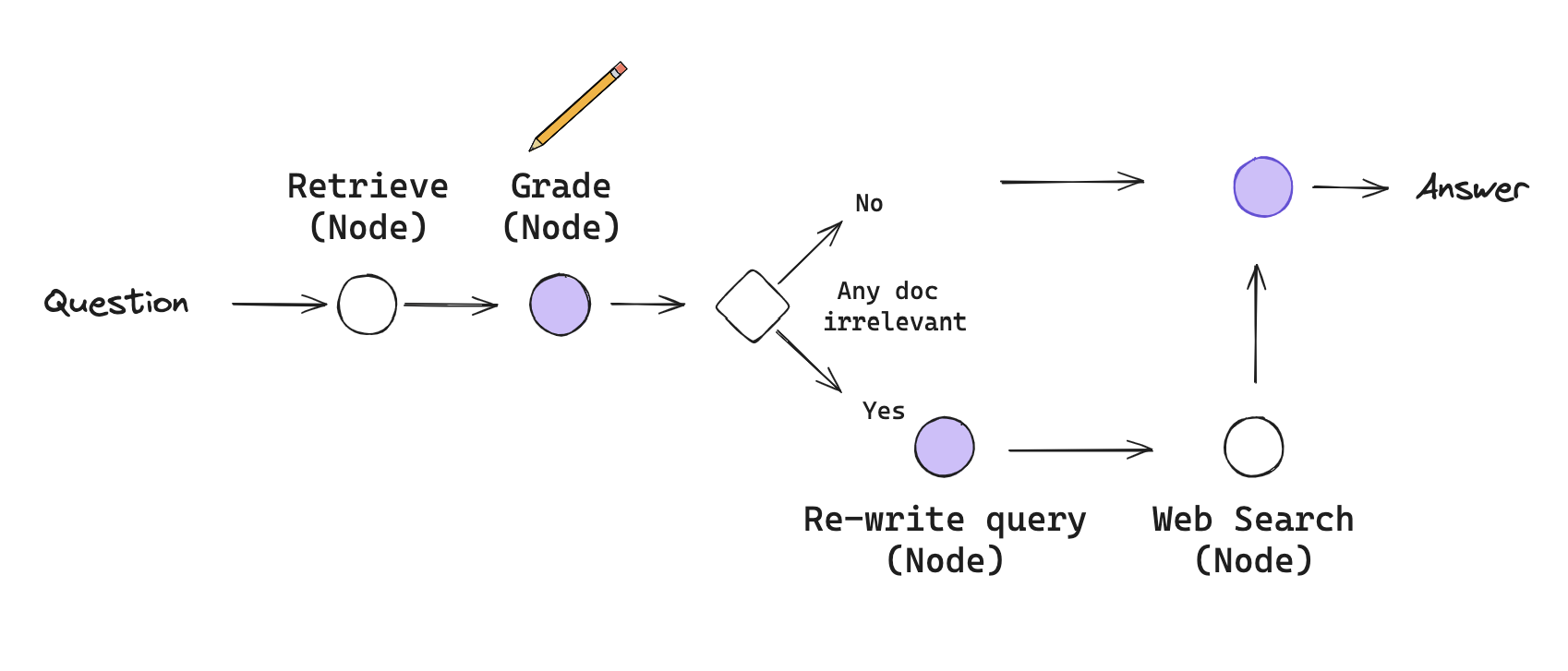
The workflow is defined by Nodes (actions) and Conditional Edges (decisions):

1. Retrieval Node: Documents are pulled from the vector store as usual.
2. Grading Node (i.e. Grader): An LLM acts as a quality control agent. It looks at the user’s question and the retrieved documents and gives a binary score: Relevant or Irrelevant.
3. The Decision Point (Conditional Edge):
   • Path A (High Quality): If the documents are relevant, the system proceeds directly to Generation.
   • Path B (Low Quality/Ambiguous): If the documents are irrelevant, the system triggers a Correction step.
4. The Correction Step:
   • Query Transformation: The LLM rewrites the user’s question to make it better suited for a broader search.
   • Web Search Fallback: The system uses a search tool (like Tavily) to find external information from the internet to replace or supplement the failed local retrieval.
5. Generation Node: The LLM generates the final answer using the best available information (either the verified local docs or the newly found web results).

Key ideas :

• Flow Engineering - This is a shift in mindset from Prompt Engineering. Instead of trying to write a single perfect prompt, you design a workflow (a graph) where the LLM performs small, logical steps and makes decisions about what to do next.
• State Machines - A CRAG pipeline is a state machine. It has a State (a dictionary containing the question, the documents, and the current plan) that gets modified as it moves through the graph. The “State” keeps track of whether retrieval was successful or if a web search is needed.
• Active RAG - Unlike Passive RAG (linear), Active RAG allows the LLM to decide :
  • When to retrieve.
  • Where to retrieve from (Vector DB vs. Web).
  • Whether the current information is “good enough” to answer.

The Corrective Power

The core strength of CRAG is its fallback mechanism. It ensures that if your internal knowledge base (Vector DB) is missing an answer or returns noise, the system can correct itself by looking at the live web, rather than just guessing.

📁 Ressources
📖 LangChain blog post : Self-Reflective RAG with LangGraph

The Context-Window Shift (Long-Context RAG)

In early 2024, RAG was a “Constraint Manager” : its job was to squeeze a big world into a tiny 32k context window. By 2026, with 1M to 10M+ token windows, the philosophy has shifted from Finding Chunks to Curating Context.

• 2024 Logic (Chunking): You split a book into 500-word pieces. You retrieve the 3 most similar pieces.
  • Result: The LLM misses the “flow” and the connections between chapters.
• 2026 Logic (Long-Context Retrieval): You retrieve entire documents or very large sections (50k–100k tokens at a time).
  • Result: The LLM has the “Big Picture” and can reason across entire themes without losing context.

Context Caching is the breakthrough that made Long-Context RAG viable in 2026.

• The Problem: Sending 1 million tokens to an LLM for every single question is incredibly slow and expensive.
• The Solution (Caching): You upload your entire 1-million-token technical manual or codebase to the LLM provider once. The provider “caches” the processed data on their servers.
• The Workflow: When a user asks a question, the LLM doesn’t “re-read” the manual. It performs an instant, high-speed search across the cached state.
• Impact: RAG is no longer a separate “Search” step; it is a “Filter” that tells the LLM which part of its massive cached memory to focus on.

The "Needle in a Haystack" Problem

While windows are huge, LLMs still suffer from “forgetting” details in the middle of a massive context. Therefore, we still use RAG techniques (like Query Translation) to help the model find the “Needle” (the fact) inside the “Haystack” (the 1M token context).

Generation

Generation is the step where the language model uses the retrieved context along with the user’s query to produce a coherent, relevant answer.

Self-RAG : Self-Reflective Retrieval-Augmented Generation

Self-RAG is a framework that trains (or prompts) an LLM to output Reflection Tokens—special tags that allow the model to critique its own retrieval quality and generation accuracy at every step.

In standard RAG, once the LLM gets documents, it just starts writing. There is no internal mechanism to stop and say, “Wait, these documents don’t actually answer the question,” or “I am making things up that aren’t in the text.”

Self-RAG uses a Self-Reflection loop powered by four specific types of evaluation:

1. Is-Retrieve: Does this query even need retrieval? (If the user says “Hi,” the model should skip RAG).
2. Is-Rel (Relevance): Is the retrieved document relevant to the query?
3. Is-Sup (Supported): Is the generated claim supported by the document? (The Hallucination Check).
4. Is-Use (Useful): Is the final answer actually helpful to the user?

Self-RAG is unique because it often retrieves multiple passages and generates multiple candidate answers in parallel, then uses the reflection tokens to pick the winner.

• Step 1: Retrieve. The system pulls $K$ number of documents.
• Step 2: Critique Relevance. For each document, the model asks: “Is this relevant?” It discards the “noise.”
• Step 3: Generate & Critique Support. For the remaining relevant documents, the LLM generates a response and then critiques it: “Did I stick to the facts in this specific document?”
• Step 4: Rank. The system scores each candidate based on its reflection tokens (e.g., this answer is 100% supported and 100% useful).
• Step 5: Final Selection. The best-ranked answer is returned to the user.

Why use Self-RAG?

• Eliminates Hallucinations: By forcing the model to check if every sentence is “supported” by the retrieved text, it significantly reduces made-up facts.
• Handles Unanswerable Queries: Because of the Is-Rel and Is-Use tokens, the model is much better at saying “I don’t have enough information to answer this” rather than guessing.
• Fine-Grained Quality: It is one of the most precise forms of RAG because it evaluates the relationship between the Question, the Document, and the Answer as three distinct steps.

The State in Self-RAG

Just like in CRAG and Adaptive RAG, the “Graph State” is critical here. The state must track the Critique Scores for each document so the final node can mathematically determine which answer is the most reliable.

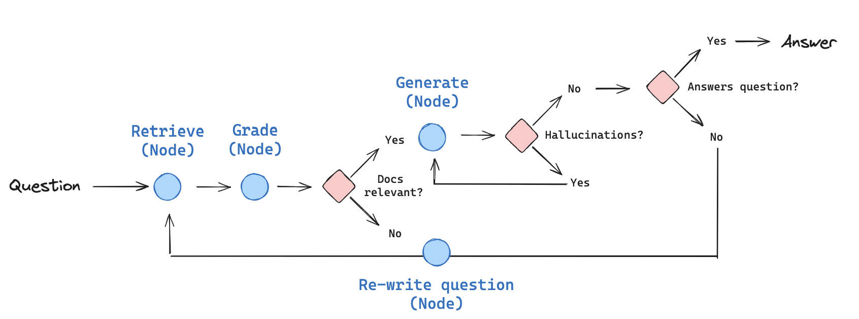
Adaptive RAG

Adaptive RAG is a self-reflective architecture. Instead of treating every question the same way, it uses the LLM as a sophisticated controller to determine the best strategy on the fly. It treats the RAG process more like Flow Engineering or Online Unit Testing.

Two core pillars :

1. Query Analysis & Routing: The Front End. The system analyzes the question before doing anything else to decide which tool or database is required.
2. Inference-Time Unit Testing: The Back End. Instead of testing the system during development, the system “unit tests” itself during the user’s request (e.g., checking for hallucinations before showing the answer).

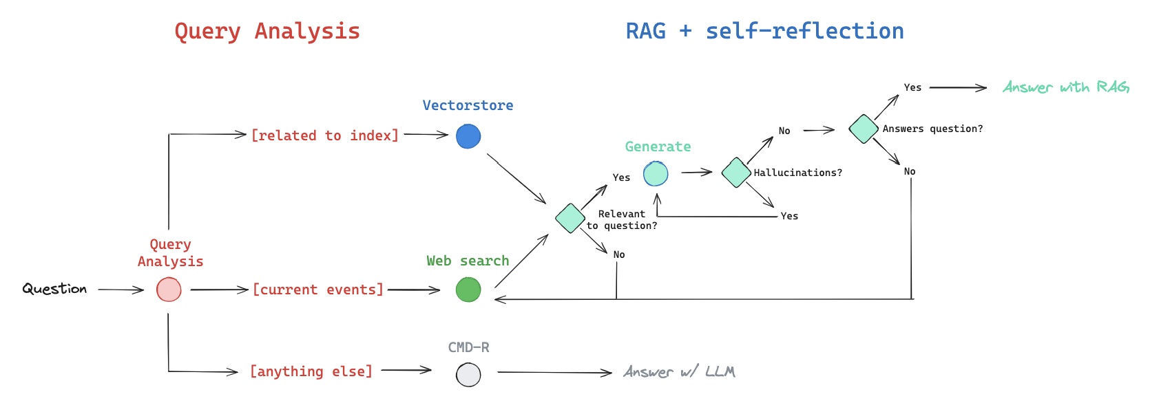
When a question enters the system, the Router chooses one of three primary directions:

• Path A : Vector Store (Internal Knowledge)
  • Use this for topics the system is specifically trained on (e.g., your company’s private docs).
  • The Safety Loop: If the retrieved documents are graded as irrelevant, the system doesn’t give up; it automatically kicks the query over to Web Search.
• Path B : Web Search (External Knowledge)
  • Use this for current events, general world knowledge, or topics not covered in the local Vector Store.
• Path C : LLM Fallback (No Retrieval)
  • For simple conversational queries (“Hi, how are you?”), the system skips retrieval entirely to save time and tokens, answering from the LLM’s internal weights.

Why use Adaptive RAG?

• Efficiency: It only uses expensive retrieval steps when necessary.
• Accuracy: It catches its own mistakes (hallucinations/irrelevance) before the user sees them.
• Reliability: By using LangGraph, the “Flow Engineering” approach ensures the system follows a logical, repeatable path, making it much more stable for production than a “free-roaming” agent.

The Self-Reflective Mindset

Adaptive RAG is essentially a system that distrusts itself. It assumes retrieval might fail and generation might hallucinate, so it builds the “correction” into the architecture itself.